NeurIPS 2023 Accepted Paper
Link: https://github.com/badripatro/svt
Summary
- 다양한 Vision Transformer-series가 많이 연구되고 있다.
- But one challenge faced by vision transformers is the increasing computational complexity of the self-attention module as the sequence length or image resolution grows
Introduction or Motivation
- Fourier-Based Transformers
- Purpose: Minimize the loss of information by using Fourier Transform.
- Examples:
- FourierFormer
- FNet
- GFNet
- AFNO
- Inherent Problem:
- Difficulty in separating low and high-frequency components.
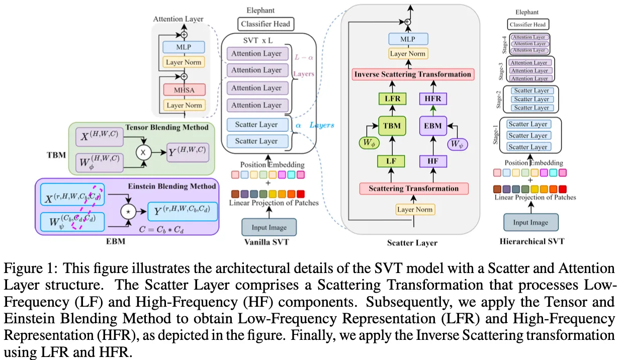
- Proposed Solution: Scattering Vision Transformer $($SVT$)$
- Components:
- Spectral Scattering Network:
- Addresses attention complexity.
- Dual-Tree Complex Wavelet Transform $($DTCWT$)$:
- Captures fine-grained information.
- Performs spectral decomposition into low-frequency and high-frequency components of an image.
- Spectral Scattering Network:
- Components:
- Frequency Component Handling in SVT
- High-Frequency Component:
- Captures fine-grained information from the scattering network using DTCWT.
- Method: Einstein Blending Method $($EBM$)$.
- Low-Frequency Component:
- Represents the energy component of the signal.
- Method: Tensor Blending Method $($TBM$)$.
- High-Frequency Component:
- Spectral Gating Network $($SGN$)$
- Function: Captures effective features in both low and high-frequency components.
- Contributions of SVT
- Utilizes TBM for low-frequency components.
- Utilizes EBM for high-frequency components.
- Characteristics of Frequency Components
- Low-Frequency Components:
- Contain the energy component of the signal.
- Require all frequency components to provide energy compaction.
- High-Frequency Components:
- Can be represented by only a few components.
- Achieved using Einstein multiplication.
- Low-Frequency Components:
Method
Discrete Wavelet Transform$($DWT$)$
- $x(t) = \sum_{n=-\infty}^{\infty} c(n) \varphi(t - n) + \sum_{j=0}^{\infty} \sum_{n=-\infty}^{\infty} d(j,n) 2^{j/2} \psi(2^j t - n)$
- $\varphi(t)$: low-pass scaling function
- $\psi(t)$: shifted version of a band-pass wavelet function
- $c(n) = \int_{-\infty}^{\infty} x(t) \varphi(t - n) \, dt, \quad d(j,n) = 2^{j/2} \int_{-\infty}^{\infty} x(t) \psi(2^j t - n) \, dt$
- $x(t)$: input
- $c(n)$: scaling coefficient
- $d(j,n)$: wavelet coefficient
- weakness:
- oscillations
- shift variance
- aliasing
- lack of directionality
- Complex Wavelet Transform $($CWT$)$
- solve the one of weakness of DWT with complex-valued scaling and wavelet function
Dual-Tree Complex Wavelet Transform $($DTCWT$)$
- Fourier Transform과 매우 유사한 특성을 가지고 있다.
- Smooth and non-oscillating magnitude
- Nearly shift-invariant magnitude with a simple near-linear phase encoding of signal shifts
- Substantially reduced aliasing
- Better directional selectivity in higher dimensions
- Real Tree
- 첫 번째 Wavelet Tree로, 일반적인 real number wavelet transform을 수행합니다.
- Imaginary Tree
- 두 번째 Wavelet Tree, Real Tree와는 약간 위상차가 있는 필터를 사용하여 복소수 wavelet을 생성합니다.
Equations
- $g_0(n) \approx h_0(n - 0.5)$
- 필터의 위상 관계
- Imaginary Tree의 low-pass filter $g_0(n)$이 Real tree’s low-pass filter $h_o(n)$을 반 샘플 시프타한 것과 유사함을 나타낸다
- 트리간의 위상 차이를 90도로 유지하여 복소수 wavelet coefficient를 형성
- $\psi_g(t) \approx \mathcal{H}\{\psi_h(t)\}$
- Imaginary Tree’s wavelet function $\psi_g(t)$가 real tree’s wavelet function $\psi_h(t)$의 hillbert transform $\mathcal{H}\{\psi_h(t)\}$ 와 유사함을 타나탠다.
- $\psi_h(t) = \sqrt{2} \sum_n h_1(n) \varphi_h(t)$
- Real Tree의 wavelet function $\psi_h(t)$는 high-pass filter $h_1(n)$과 scaling function $\varphi_h(t)$의 합성으로 정의
- $\varphi_h(t) = \sqrt{2} \sum_n h_0(n) \varphi_h(t)$
- Real Tree의 scaling function $\varphi_h(t)$는 low-pass filter $h_0(n)$와 자신의 다운샘플링된 버전의 합성으로 정의
Scattering Transformation
- Via DTCWT
- Fine-grain information:
- Consists of texture, patterns, and small features.
- Encoded by the high-frequency components of the spectral transform.
- Global information:
- Consists of overall brightness, contrast, edges, and contours.
- Encoded by the low-frequency components of the spectral transform.
- Frequency representations: $\mathbf{X}F=\mathcal{F}\text{scatter}(\mathbf{X})=\mathbf{DTCWT}({\mathbf{x})}$
- $\mathbf{X_F}(u, v) = \mathbf{X_\varphi}(u, v) + \mathbf{X_\psi}(u, v)\\~~~~~~~~~~~~~~~~= \sum_{h=0}^{H-1} \sum_{w=0}^{W-1} c_{M,h,w} \varphi_{M,h,w} + \sum_{m=0}^{M-1} \sum_{h=0}^{H-1} \sum_{w=0}^{W-1} \sum_{k=1}^{6} d_{m,h,w}^{k} \psi_{m,h,w}^{k}$
- $\mathbf{X_\varphi}(u, v)$: 저주파 성분(approximation coefficients)을 사용하여 재구성된 신호
- $\mathbf{X_\psi}(u, v)$: 고주파 성분(detail coefficients)을 사용하여 재구성된 신호
Spectral Gating Network
- extract spectral features from both low and high-frequency components of the scattering transform
- use learnable weight parameters to blend each frequency components
- Tensor Blending Method $($TBM$)$ for low-frequency
- 저주파수 성분 $\textbf{X}\varphi$과 학습 가능한 가중치 $\textbf{W}\varphi$를 요소별 텐서 곱셈(Hadamard multiplication)을 사용해 혼합
- 이미지의 전역 정보(예: 밝기, 대비, 가장자리)를 캡처
- $\mathcal{M_\varphi} = [\mathbf{X_\varphi} \odot \mathbf{W_\varphi}], \quad \text{where } (\mathbf{X_\varphi}, \mathbf{W_\varphi}) \in \mathbb{R}^{C \times H \times W}, \text{ and } \mathcal{M_\varphi} \in \mathbb{R}^{C \times H \times W}$
- Einstein Blending Method $($EBM$)$ for high-frequency
- 이미지의 세밀한 정보(예: 텍스처 및 작은 세부 사항)를 캡처
- 파라미터 수와 계산 비용을 효율적으로 제어
- EBM 수행 단계:
- 텐서 $A$를 $\mathbb{R}^{H \times W \times C}$ 에서 $\mathbb{R}^{H \times W \times C_b \times C_d}$로 reshape.
- 여기서 $C = C_b \times C_d$ , $b \gg d$ .
- 텐서 $A$를 $\mathbb{R}^{H \times W \times C}$ 에서 $\mathbb{R}^{H \times W \times C_b \times C_d}$로 reshape.
- 가중치 행렬 정의:
- 크기가 $\mathbb{R}^{C_b \times C_d \times C_d}$인 가중치 행렬 $W$를 정의.
- 아인슈타인 곱셈$($Einstein multiplication$)$ 수행:
- 텐서 $A$와 $W$를 마지막 두 차원에서 곱해 혼합된 특징 텐서 $Y$ 생성.
- 결과 $Y$는 $\mathbb{R}^{H \times W \times C_b \times C_d}$
- EBM 공식:
- $\mathbf{Y}^{H \times W \times C_b \times C_d} = \mathbf{A}^{H \times W \times C_b \times C_d} \ast \mathbf{W}^{C_b \times C_d \times C_d}$
Spectral Channel and Token Mixing
- EBM을 spectral channel에 적용한게 Spectral Channel Mixing
- $\mathbf{S_{\psi_c}}^{2k \times H \times W \times C_b \times C_d} = \mathbf{X_{\psi}}^{2k \times H \times W \times C_b \times C_d} \ast \mathbf{W_{\psi_c}}^{C_b \times C_d \times C_d} + b_{\psi_c}$
- EBM을 token-level에서 수행하는게 Spectral Token Mixing
- $\mathbf{S_{\psi_t}}^{2k \times C \times W \times H} = \mathbf{S_{\psi_c}}^{2k \times C \times W \times H} \ast \mathbf{W_{\psi_t}}^{W \times H \times H} + b_{\psi_t}$
Experiment

'AI' 카테고리의 다른 글
| FS-DETR: Few-Shot Detection Transformer with prompting and without re-training (0) | 2024.11.17 |
|---|---|
| Enhancing Ultra High Resolution Remote Sensing Imagery Analysis with ImageRAG (0) | 2024.11.14 |
| SpectFormer: Frequency and Attention is what you need in a Vision Transformer (0) | 2024.11.06 |
| Inception Transformer (0) | 2024.11.06 |
| OmniSat: Self-Supervised Modality Fusion for Earth Observation (0) | 2024.11.06 |
